Probability and Statistics Cookbook

A great resource -- Matthias Vallentin has assembled this "Probability and Statistics Cookbook", full of formulas, functions, and graphs.

-30-

Actuarial baseball

Been off the grid for a while...

A couple of weeks ago, Josh Hamilton of the Rangers hit a grand slam that got an above-average amount of attention, since it was tied into a promotion being run by a flooring company.  The title of this article describing the homer could instead be "Josh Hamilton's grand slam yields big insurance payout":
http://espn.go.com/dallas/mlb/story/_/id/6971469/texas-rangers-josh-hamilton-slam-triggers-free-flooring-payout

Somebody, somewhere, in some insurance company, sold coverage for this promotion.  And that same somebody (we hope) must have sat down and calculated the probability of Hamilton hitting a grand slam over a one month period, and set the premium based on that probability.

Summary:  insurance is gambling.

-30-

Early season standings and Bayes

Early season performance has been a hot topic this year (not that it isn't a topic of discussion every year).  I wrote about it, using a simple approach of assuming that every team is .500, and a more recent addition in the blogosphere is Rob Neyer's take.

Last week Kincaid over at 3-D baseball had great post that used Boston's 2-10 start to go down a detailed and more sophisticated Bayesian path to estimating the team's true talent.  Tango posted a link to Kincaid's blog, and added a few details that incorporate actual observations.  A key element in this is that the observed spread of talent is wider than the theoretical .500 level of all teams.  (If all teams were .500, the random component would result in a standard deviation of 0.039. In reality, the standard deviation is wider, at 0.071 -- the implication of this is that there are real talent differences between teams, with some teams having a true talent level above .500 and others below.)

My modest contribution to this thread is here:  a Google doc spreadsheet that show all of the MLB team's current record (as of 2011-04-30), and then takes two different Bayesian-based methods to predict each team's final season outcome.

The first set are the yellow columns, which replicate Kincaid's "shortcut" approach, with the implied regression of 69 games noted by Tango. The blue columns take a different approach that uses the standard deviation of both the observed performance to date and the long-term observations (every MLB team season outcome from 1961-2010) as the prior.

The difference in the result generated between these two approaches is relatively modest.  (It's worth noting that the relative position on the standings does not change.) What is apparent is that with roughly 25 games played this season, there are solid differences appearing in the team performances.  This method forecasts that Cleveland and Philadelphia will regress downward from .692 (a 112 win season) to .573 and end up with 93 wins. At the bottom of the table, it suggests that the Twins will improve from .346 (58 wins on the season) to .444 and a much more respectable 74 wins over the course of the season.

-30-

Words with meaning

Article at Slate entitled "Turning words into touchdowns", on the work of Achievement Metrics. This company takes interviews from various players and parses them, and then correlates the pattern with on- and off-field performance.  From AM's website:

Our analyses of players’ speech, arrest, and suspension data have shown that differences in players’ speech while in college can predict which players are more likely to exhibit off- and on-field behavioral problems during their professional careers.

I'm not sure whether this would work for baseball, since the players just speak in clichés. (Warning: clip includes profanities.)

-30-

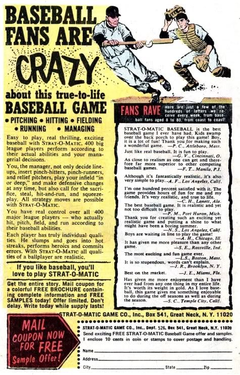
Baseball fans are crazy

Or so says this ad for Strat-o-matic, posted at If Charlie Parker was a Gunslinger...
 (Note: the main Charlie Parker page is not appropriate for at-work viewing.)

(Click the image to enlarge.)

-30-

On pace for a 162 loss season!

Two days ago I responded to an on-line article about the Orioles' 4-0 start to the season, pointing out that it's not at all surprising -- using the laws of binomial probability -- to see three of the 30 MLB teams at 4-0 to start the season.

What I didn't mention were the teams that started the season on a losing streak. And now, heading into this weekend's play, the 0-6 Red Sox and Rays that are getting the attention of the punditocracy.  For the Red Sox, it's the poorest start since the 1945 season, and the Rays haven't ever gone 0-6 to start the season in their comparatively short history.

Some writers have acknowledged the probability and the history of being 0-6:  Dave Cameron at FanGraphs writes "Is it time to panic in Boston?", and Cliff Corcoran at S.I.'s piece is "It's still early, but history is against winless Red Sox, Rays and Astros" (which was written before yesterday's games, when the teams were 0-5).

An entirely different view can be found Baseball Prospectus, where Steven Goldman uses the 1987 Brewers, who went 13-0 and then 20-3 (Goldman writes, "on pace for a 141 win season") before hitting a 12 game losing streak, and the opening sequence of Tom Stoppard's existentialist play Rosencrantz And Guildenstern Are Dead to suggest that sometimes things operate outside the laws of probability.

(Watch the scene in question, from the 1990 film with Gary Oldman and Tim Roth as the title characters.)

In the play, the characters are faced with a preposterously long string of coin-flips that land heads. This leads Guildenstern to say "A weaker man might be moved to re-examine his faith, if in nothing else at least in the law of probability."

Even though the two teams are 0-6, the weakness of my faith in the laws of probability is not yet tested.

-30-

On pace for a 162 win season!

Only at the beginning of the season would a four-game winning streak get you an article on S.I.

The probability of a true .500 team playing four games against other true .500 teams and winning them all is 6.25% -- or roughly 2 out of 30. In other words, at this point in the season we could realistically expect two teams to be at 4-0.  Once we consider that in real life teams are not so perfectly matched, thus raising the odds of the more powerful team being successful in all four games, the fact that there are three teams with 4-0 records (Orioles, Reds, and Rangers) isn't a surprise.

The only surprise in all of this is that the Orioles (widely touted to finish last in the A.L. East) swept the Rays in a three game series in Tampa Bay and then went on to beat the Tigers at home in their fourth game of the season. But then again, the probability of a .400 team going 4-0 against a .500* team is just under 3%.  Not very good odds, but something we would expect to see on occasion.

(Shout out to Tango, who raised the "on pace" problem a couple of days ago, and The Book readers who added various lucid and perceptive comments, including an XKCD cartoon. You can never go wrong using an XKCD cartoon to illustrate your point.)

Update: the New Utosky Bolshevik Show takes the Red Sox 0-3 start as its jumping off point for a post titled The Red Sox Aren't Doomed, demonstrating the same thing I did but with graphs and Python script.  Score one for the NUBS.

* Changed from ".600".  Comment #1 below was generated because of this typo; #2 is my detailed response.

-30-

The ERA distribution curve

NOTE: Tango and MGL at The Book, through the "Lemonade" thread, have critiqued the analysis below and pointed out errors in my assumptions. These errors mean that my closing conclusions are wrong -- good math, but bad statistics on my part. Through this post, you will find italicized text describing my errors.
Revised January 5, 2011

---

J.C. Bradbury's recent blog postings (here and here) have included histograms showing the distribution of ERA across major league pitchers for the 2009 season.  For his analysis, Bradbury omitted those pitchers with fewer than 100 batters faced -- in both his blog and book Hot Stove Economics, he justifies this due to the wide variance in ERA scores, much of which will be due to the small number of "samples" for each pitcher.  (As we saw in my earlier post about Bo Hart, it's possible for an average player to do very well over the short term; the inverse applies too.)

But a few comments on Bradbury's blog from readers ask about the impact that those "missing cases", who account for nearly a third (28%) of all individuals who pitched in MLB in 2009, would have on the curve.

Here's the answer: 

Figure 1: MLB Pitching, 2009 -- Number of Pitchers by ERA, by Number of Batters Faced

Incorporating the <100 BFP pitchers (the black chunks of each bar) adds pitchers across the whole range, although they are skewed to the right (i.e. higher ERAs).  While there is a stack on the left with very low ERAs, there's a bigger group of players with an ERA greater than 10. (The highest ERA of this group was 135.00.)

NOTE 1: ERA is a poor measure to use for this type of evaluation -- for pitchers with a low number of batters faced or innings pitched, it's easy for huge numbers to appear. That 135.00 ERA is the equivalent of 15 earned runs with only a single recorded out.  These exaggerated values then lead to an upward distortion of the mean for the group.  A better measure would be wOBA, or other measure that resembles a probability between 0 and 1.

The table below shows the average ERA of this group and three other groups based on the number of batters faced.  What we see is that the <100 BFP pitchers have a higher ERA than those who pitched more frequently.  (This difference is statistically significant.)  In spite of the variation in their ERAs, this group on average are less skilled than the other three groupings of pitchers.

NOTE 2: This is where I went wrong. The math is correct, but there is bias in the sample that I ignored. We can be fairly confident that pitchers who get off to a poor start won't get many opportunities to pitch -- and therefore won't get the opportunity to regress to the mean. Pitchers who do better at the start of their season will continue to pitch, and regress to the mean.  This process may take them some time, which may push them over the arbitrary line of 100 batters faced.  Thus the statistical significance is an artifact of the bias.

Figure 2: MLB Pitching, 2009 -- Average ERA, by Number of Batters Faced

In a thread on The Book blog that covered this same topic, I made a similar statement (reply #8): "What I’m trying to say is that our best estimate of the “true talent” of this group is an ERA of 8.11 [in the current case, 8.72], and that estimate is quite accurate". That statement got a response from Tango (reply #9) of "That is not accurate. If you look at how those pitchers who faced fewer than 100 batters did in the season preceding or the season following, THAT will give you a much better indicator of the true talent level."

So let me clarify.  The average level of skill of the pitchers who faced fewer than 100 batters in 2009, is an average ERA of 8.72. Although Tango is correct in his assertion that the poorest performers would regress upwards, by the same token the best pitchers (some of whom managed a 0.00 ERA in their short stint) would get worse. But if we were to let all 188 of them continue to pitch, we can be 95% certain that the "true" ERA of the group would end up somewhere between 6.92 and 10.52.

Even the lower bound (i.e. the lowest score we would expect with our more rigorous testing) is higher than the highest range from the other groups.

NOTE 3:  My statement above would be correct, if it were not for the bias in the sample.  My belief had been that this group would regress not to the MLB average, but to the average of the <100 BFP pitchers.  But because of the selection bias, this does not hold true.
Here's a simple example to demonstrate how this works. Think of the probability professor's favourite tool, the coin toss. If we have a penny and toss it repeatedly -- say, 10,000 times -- and recorded the result each time, the proportion of heads would very accurately reflect the true probability of the individual penny. And we'd need plenty of tosses to get an accurate measure of the single penny.

But what if instead of one penny we had 188 pennies, and we varied the number of tosses each penny got? Although the average number of tosses would be 50, some pennies might get only one toss, while others would get as many as 100 tosses. Some of those short sequences might come up all heads, while others would heavily favour the tails. On average, though, across the 188 pennies, we would find that the group average was a close reflection of "true average" of the group.

NOTE 4: The error in the initial assumption causes my coin flipping analogy to fall apart.  If “success” is a head, then the coin that comes up heads >0.5 will keep being flipped, possibly with enough flips to no longer be part of the “low flip” group (over that arbitrary threshold).  Meanwhile, a coin that runs tails more often will get pulled from the trials quickly, and end up <0.5 and with few flips.  Thus, as a group, the coins with a smaller number of flips will end up looking worse than those that keep getting flipped.  Selection bias causes an apparent difference, where none really exists.


And so it is with the pitchers in question. If they were like the other pitchers in MLB, we would expect that some of the <100 batters faced pitchers would have ERAs above the league average, while others would fall below. What we see, however, is that while there is a wide variation, the average is substantially higher than the other groups of pitchers.

NOTE 5:  ...because of selection bias!  The lesson:  selection bias can crop up anywhere, even if you are not the one doing the selecting.

-30-

Graphing run expectancy

Baseball Prospectus provided the world with the 2010 situational run expectancies, and Joshua Maciel has provided a graphic display. The graph was first posted to and then evolved as a result of feedback from readers at Tango's blog -- a fascinating process in and of itself. The graph is still a bit busy to my mind (but it's certainly not a Tufte-ian duck...), but it's a fine piece of work displaying what is arguably one of the most important pieces of baseball data.

And remember, it was George Lindsey who first published these data, back in 1963.

[Right: Joshua's run expectancy chart. Click to see it full-size, and visit his blog for all the details.]

-30-

Bo knows probability

Cardinals' second baseman Bo Hart

Over on 3-D Baseball, Kincaid has a nice explanation of regression to the mean in a post titled "On Correlation, Regression, and Bo Hart". The blog entry starts with the story of Bo Hart, who got called up to the Cardinals in June 2003, and promptly hit .412 over his first 75 at-bats. Since Kincaid wrote a regression to the mean article, you can guess where Hart's season went -- he finished with 286 at-bats and a .277 average.

But Kincaid flirts with a few notions that I think are worth following in a bit more detail.

First up, what are the odds that a .277 hitter will break .400 across a string of 75 at-bats?

The answer is roughly 1 in 200.

This is calculated through the fact that the binomial distribution approximates the normal distribution -- in English, if you repeat a set of binomial trials, the histogram of the count of success rates for the trials will look like the normal curve. This leads us to the probability density function, which allows us to state the probability that a value (in this case, a batting average of .412) falls at a certain point given the mean value (.277).

Using Bo Hart's season batting average of .277 as his "true talent" (or "population mean") across 75 at-bats, we can calculate the standard deviation of the distribution (0.052). We then determine that .412 lies at 2.60 standard deviations from the mean (2.60=[.412-.277]/.052). As a probability, 2.60 standard deviations is 0.5% -- or 1 in 200.

What was unusual about Bo Hart is that his 1 in 200 string of successful at-bats occurred at the beginning of his Major League career. Calculating that probability is a task for another day.

In my next post I will explore Kincaid's statements about evaluating "true talent" based on a number of observations. Specifically, I'll delve into the following questions: "At what point can we be relatively certain about our inferences of true talent based on observed performance? 75 PAs is not enough, and one million is plenty, but what about 1000?"

-30-

Skill, luck, and more than a little style

Pictured: "Mr. May", Dave Winfield, comes through in the clutch in the 1992 World Series with, in his words, "One stinkin' little hit." The 11th-inning double drove in two runs and sealed the World Series win for the Blue Jays.


The BBC has posted an article and calculator ("Can chance make you a killer?") that is used to demonstrate the challenges in differentiating luck from skill. In this case, a simple scenario with fixed parameters is linked to a calculator that generates the range of possibilities.

While I'm not sure how this could be used in a baseball setting, it is a very good tool for demonstrating that it can be difficult -- particularly if you just look at "the numbers" in a selective way -- to make definitive statements about a player's ability. Such as, say, clutch hitting.

(Acknowledgement: The Book.)

Tireless tennis

After a bit of water-cooler chat today at work, I had planned to spend part of my evening working out the probability of the crazy Wimbledon match that saw John Isner win a marathon match against Nicolas Mahut, after the tie-breaker went 138 games and had Isner prevail 70-68.

I got home to find not one but two well-presented analyses that tackle the question, so my work would be redundant. Thus I present the following links for your reading pleasure:

1. Carl Bialik, "Isner Fitting Winner of Marathon Wimbledon Match", Wall Street Journal

2. Phil Birnbaum, "What were the odds of the 70-68 score at Wimbledon?", Sabermetric Research. (Birnbaum graciously acknowledges Bialik's article in an appended post-post foreward.)

The final summary: this was a one-in-a-million (give or take, depending on some of the assumptions) event.

Perfectly random?

There has been much discussion about the recent run of perfect and almost-perfect games. A variety of hypotheses have been floated, including
pitching dominance (including a higher strike out ratio), improved defense, and the confluence of expansion, better player evaluation, and a drug-free world.

Perfect games are a rare event, so we run the risk of seeing a random cluster as a trend. There have now been 20 perfect games -- 18 in the "modern era" (since 1900), 14 since the expansion era began in 1961, and two so far in the 2010 season. How can we tell if this "streak" of two perfect games in a single season is simply a random fluctuation?

Calculating the probability of a perfect game: allowing runners

One approach is to calculate a theoretical probability based on on-base percentage (OBP). Tango has a blog entry "Perfect Game calculation" that presents one approach. His estimate was 1 perfect game per 15,000.

Another example of this appears in Mathletics by Wayne L. Winston, who calculated a probability of 0.0000489883, or 1 game in just over 20,400. Winston noted at the time the book went to press (before the 2009 season) there had been nearly 173,000 regular season games since 1900 and each game provides 2 opportunities for a perfect game (so we have 346,000 "team games"). Winston then goes on to note that we would therefore expect there to be 16.95 perfect games over that period -- almost perfectly matching the observed total of 17 to that point in time.

A side note: after Mark Buehrle's perfect game in 2009, Sky Andrecheck took a similar approach for individual players. He worked out the individual chances for the 16 modern-era players who had tossed a perfect game, based on the sum of the on-base percentage and reached-on-error percentage they allowed over their careers.

Calculating the probability of a perfect game: observed rate

A second approach to calculating the probability is to compare the observed number of perfect games and to the number of opportunities. I decided to use 1961 as year one. This was a natural point to begin -- this was the first year of baseball's expansion, and it falls mid-way between Don Larson's 1956 World Series perfecto (which had been the first in 22 years) and Jim Bunning's 90 pitch masterpiece in 1964. Between 1961 and 2009 inclusive, there were 12 perfect games -- and there were 201,506 regular season "team games". This gives us a probability of 0.00005955, or 1 perfect game every 16,790 team games played.

This method yields a result that is roughly the mid-point between Tango's and Winston's approaches.

What are the odds of two perfect games in one season?

While most statistical analysis makes the assumption that the distribution of the events is "normal", when we are dealing with rare discrete events the distribution does not resemble the normal distribution. The most common distribution used for this is the Poisson distribution.

At the probability of 1 in 16,790 across a season of 4,860 "team games" (the current number per season -- based on 2,430 games and therefore 4,860 perfect game opportunities) and 4,112 (the average number since 1961) that the probabilities, expected frequencies, and observed frequencies are as follows:







So over 50 seasons, we would predict that there would be between 1 and 2 seasons with 2 perfect games, and between 9 and 11 seasons with 1 perfect game.

So to answer the question posed in the title, the answer is "Yes -- two perfect games in one season is well within the expected distribution." The fact that 2010 has been the first season with 2 perfect games in the 50 years since 1961 fits perfectly with the expected distribution.


In future posts I will repeat the calculation of probabilities and frequencies, with modified probabilities (once the dust settles on the "correct" way to calculate the probabilities...)

Comments and questions are always welcome.